Category: AI & Open Source

  • Liquid AI Releases 24B MoE with 2B Active Params per Token

    Liquid AI Releases 24B MoE with 2B Active Params per Token

    Liquid AI has unveiled LFM2.5-24B-A2B, a Mixture-of-Experts (MoE) reasoning model that activates only 2B of its 24B parameters per token. According to an announcement published on the Hugging Face blog dated October 13, 2026, the model is designed to perform explicit thinking before producing an answer, invoke tools, and execute multi-step tasks within agent harnesses such as OpenClaw, Hermes Agent, Pi, and OpenCode. Because active parameters are limited to 2B per token, the per-inference-token cost is low, positioning the model as an on-device AI option for continuously running agents on self-owned hardware.

    Architecture: 40 layers, 64 experts, hybrid attention

    LFM2.5-24B-A2B inherits the LFM2-24B-A2B design with 40 layers, 64 experts per MoE block, and top-4 routing, retaining the same hybrid attention of gated short convolutions and GQA (Grouped Query Attention). The context window has been expanded from 32K to 131K tokens, and the tokenizer’s vocabulary has grown from 65K to 128K, improving non-Latin tokenization. Unlike LFM2-24B-A2B, it operates as a reasoning-only model and produces an explicit Chain of Thought before its final answer.

    Training pipeline: 33T pre-training and 5-stage post-training

    Pre-training token count has increased from approximately 17T to approximately 33T. Mid-training consists of 2T tokens at 32K context weighted toward reasoning, math, code, instruction following, and multilingual text, plus 300B tokens at 131K context weighted toward long-context data, with tool-calling and multi-turn trajectories appearing across both stages. Post-training proceeds in five stages: ① supervised fine-tuning (SFT); ② Multi-domain On-Policy Distillation (MOPD) non-agent stage, distilling expert models into non-agent tasks; ③ MOPD agent stage, distilling agentic tasks; ④ agentic reinforcement learning (training inside the agent harness); ⑤ follow-up fine-tuning.

    Agent performance: #1 in 5 tool-use and 3 instruction-following benchmarks

    Evaluation was conducted with vLLM, comparing against Qwen3.6-35B-A3B, Gemma-4-26B-A4B-it, and Nemotron-3.5-Lightning across 16 benchmarks spanning tool use, agentic workflow, knowledge, instruction following, math, and coding. Despite being the smallest model in the group, LFM2.5-24B-A2B delivered competitive performance against MoEs with roughly 50% more total and active parameters. Among the eight tool-use and agentic benchmarks, it ranked first or tied for first on five — AutomationBench, BFCLv4, ToolSandbox, LiveClaw, and τ³-Bench Banking — and on AutomationBench it scored more than three times the next-ranked model. On LiveClaw it scored 48.09, ahead of Qwen3.6-35B-A3B’s 38.19, and it also took first place across all three instruction-following benchmarks. On the other hand, larger models maintained their edge on knowledge-centric benchmarks such as GPQA Diamond, HLE, and AA-Omniscience, and on coding benchmarks such as SWE-Bench Verified (OpenCode) and SciCode.

    Inference speed: 184 tok/s on M5 Max, 21K tok/s on a single B300

    The model is supported out of the gate on llama.cpp, MLX, vLLM, SGLang, and ONNX. On edge inference, it recorded decoding speeds of 184 tokens/s on Apple M5 Max and 114 tokens/s on Ryzen AI Max+ 395, while using the least memory — up to 1.7× faster than the next-ranked model. On GPU inference, a single NVIDIA B300 broke through 21K output tokens/s under high concurrency, delivering the fastest speed in its size class.

    Benchmark / Environment LFM2.5-24B-A2B Comparison
    LiveClaw (agentic composite) 48.09 Qwen3.6-35B-A3B 38.19
    Edge decoding (Apple M5 Max) 184 tokens/s Up to 1.7× next-ranked
    Edge decoding (Ryzen AI Max+ 395) 114 tokens/s Up to 1.7× next-ranked
    Datacenter GPU (single B300) 21K tokens/s (high concurrency) Best in class

    Practical integration steps and agent harness linkage

    The model is connected by serving it locally as an OpenAI-compatible backend and then pointing an agent harness at it. It is loaded through AutoModelForCausalLM in transformers 5.0.0 or later, with device_map=auto, dtype=bfloat16, and the flash_attention_2 option on compatible GPUs. In Hermes Agent, model.provider is set to custom, model.base_url points to the local OpenAI-compatible endpoint, and model.context_length is set to 131072 to enforce tool use. Default ports per serving backend are 8080 for llama.cpp and MLX, 8000 for vLLM, 30000 for SGLang, and 1234 for LM Studio. Because they share the same OpenAI-compatible interface, the same procedure can launch an agent on laptop-class edge devices such as the M5 Max, extending on-device AI applicability from data centers to personal devices.

    Limitations and implications

    In knowledge- and coding-oriented workflows, larger models still hold the advantage, and combining RAG or web search is recommended. The combination of 131K context and a 2B-per-token active parameter structure targets on-device AI scenarios that process tool calls and multi-step reasoning locally without external API dependencies. With both LFM2.5-24B-A2B and LFM2.5-24B-A2B-Base released as open weights on Hugging Face, the model is regarded as worth immediate review by teams that want to operate private agents on their own hardware.

    Reference

    This article was prepared by checking the following source: Hugging Face Blog — Run fast, private agents on-device with LFM2.5-24B-A2B

  • Open-Weight LLMs and Secure Enclaves Replace ChatGPT

    Open-Weight LLMs and Secure Enclaves Replace ChatGPT

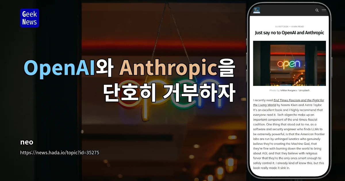
    Closed frontier models from OpenAI and Anthropic have dominated the LLM market as the de facto standard. However, growing concerns in practice revolve around the fact that neither company effectively relinquishes access to conversation data through a simple training-opt-out toggle, and that loosely guarded model access may have been granted to certain U.S. cybersecurity firms and defense contractors. As a result, the search for alternatives to break this dependency in real-world environments is accelerating. The core of these alternatives lies in open-weight models and private inference services built on secure enclaves.

    Training opt-out settings are not a privacy guarantee

    OpenAI and Anthropic offer their most powerful models only as closed services, and users pay for chat or API access. Even when the training opt-out toggle is enabled, both companies retain full access to conversations and can review them or share them with governments and enterprises. This shows that training opt-out and private conversations are fundamentally different concepts. Even if both companies are currently likely to respect the opt-out, that alone is not enough to ensure long-term trust in how data is handled.

    In the cybersecurity domain in particular, strict guardrails are applied. Agents that monitor conversations block session activity when they detect potential hacking behavior, but this approach is frequently criticized for producing false positives. On the other hand, certain users are granted model access with loose or no restrictions, and it is estimated that access may extend to multiple U.S. cybersecurity firms, almost certainly U.S. defense contractors, and any U.S. government agency that wants it. While restricting powerful models has some legitimacy, critics argue that leaving final access decisions to Sam Altman and Dario Amodei, who then coordinate with the executive branch, is undemocratic.

    How far have open-weight models come?

    Open-weight models are analyzed to lag roughly four months behind OpenAI and Anthropic’s advanced proprietary models, and this gap is considered small. GLM-5.3 is reported to perform roughly on par with Claude Opus 5.5 in software engineering, and the smaller GLM-5.3-Flash is evaluated as comparable to Claude Opus 4.8. If one can obtain a Mac Studio with 512GB of RAM, running GLM-5.3 locally as an individual is a realistic option.

    However, the usefulness of a model and the trustworthiness of its developer as a data custodian are separate questions, and creating an account directly with Z.ai, GLM’s developer, or sending data to it is not recommended. Given that ZCode, the coding harness corresponding to Claude Code, was recently found to have uploaded local source code repositories to Alibaba Cloud without user consent, it is safer to assume that data provided to Chinese companies can be shared with the Chinese government. DeepSeek, Qwen, and Kimi families are also cited as impressive open-weight models, but the same distinction applies: relying on their developers as data custodians for conversations should be treated separately.

    French company Mistral is classified as the only major LLM developer that is neither an American nor a Chinese company, and the nickname of its new frontier model Mistral Large 4 is Le Chonk. Entrusting data to Mistral rather than to an American or Chinese company is considered considerably more reasonable.

    How secure enclaves reshape private inference

    Secure enclave-based inference enables private AI use without local hosting. It is not perfect, but it provides a meaningful privacy difference compared with providers having unrestricted access to all data. Tinfoil is cited as the company working most actively in this space, with technical details available in its secure enclave and remote attestation documentation. Maple AI is another alternative, internally using Tinfoil’s inference service.

    By use case, Tinfoil is recommended for serious agentic coding work such as software engineering, reverse engineering, malware analysis, CTF, and penetration testing, and charges for private inference based on token usage with no monthly subscription. Maple is positioned for general consumers who want a ChatGPT-like experience, including chatbot conversations, web search, document access and processing, and mobile apps, with a small free tier and a $20/month Pro plan.

    For those who do not want to pay extra for private inference, an inference router like OpenCode Go is an option. OpenCode Go costs $10 per month and provides credits that exceed $10, with requests passing from the user’s computer through the OpenCode Go API to the actual inference provider. However, both OpenCode Go and its backend providers can access session data, and while GLM, Qwen, Kimi, and DeepSeek models are explicitly listed as zero-day retention targets, this is only a policy promise and not technically guaranteed.

    Comparing private and low-cost inference options

    Item Tinfoil Maple AI OpenCode Go
    Core approach Secure enclave-based private inference Internally uses Tinfoil inference Inference router, connects to various backends
    Recommended use Agentic coding, reverse engineering, penetration testing Chatbot, search, document processing, mobile Low-cost routing for mostly public work
    Pricing No monthly fee, token-based usage Free tier + $20/month Pro $10/month + credits exceeding $10
    Privacy guarantee Technically reinforced via secure enclaves Private via Tinfoil backend Zero-day retention policy (not technically guaranteed)
    GLM-5.3 unit price Input $1.80 / cached $0.80 / output $5.75 (per 1M tokens) Same inference backend Same rate via router

    Practical workflow: OpenCode + Tinfoil + GLM-5.3

    Connecting Tinfoil and OpenCode Go to the coding harness OpenCode simultaneously and using GLM-5.3 mostly at a low inference level has been introduced as a real-world applied case. The inference provider is split depending on whether the work is public: fully public tasks, such as feature implementation for already open-source code, use OpenCode Go, while all other tasks use Tinfoil.

    GLM-5.3’s token pricing is $1.80 per million tokens for input, $0.80 for cached tokens, and $5.75 for output, and reports indicate that setting a low inference level significantly reduces token usage while still delivering impressive results. In practice, evaluations describe costs as similar or lower, privacy as higher, and guardrails as far fewer. However, the pace of model change is fast, and what constitutes the best choice six months from now is unknown.

    In early use cases, open-weight models appear to fully replace ChatGPT and Claude, and the ability to choose the runtime environment and provider itself acts as a practical insurance against single-vendor lock-in. As the ZCode unauthorized upload case shows, the data custodian trust issue remains an area that must be evaluated separately from model selection when choosing a coding harness.

    Reference source

    This article was written after verifying the following original: geeknews — Resolutely rejecting OpenAI and Anthropic

  • vLLM Decision 3.0: 5 Multimodal Decision Models, 0.8B–27B

    vLLM Decision 3.0: 5 Multimodal Decision Models, 0.8B–27B

    The vLLM project’s Semantic Router team has released the ‘Decision 3.0‘ decision model family under the Apache-2.0 license, covering 0.8B–27B parameter scales and skipping the text generation step entirely. According to the October 11, 2026 announcement, the five models were fine-tuned from the Qwen3.5 and Qwen3.8 families and process text, JSON, and image inputs in a single forward pass, returning responses as normalized probability distributions. This approach, named the ‘System One’ routing pattern, appears to be a structural attempt to lower the cost of intent classification, guardrails, and branching decisions in agent systems.

    Lineup Composition and Open Source Policy

    The Decision 3.0 family consists of five sizes: d3-lite (0.85B), d3-nano, d3-mini, d3-flash (9B), and d3 (26.09B). The announcement states that all models are distributed under Apache-2.0 and only BF16 weight precision is provided. No separate quantized variants are available on official channels, so users must choose directly from 0.85B to 27B based on VRAM headroom.

    The base models are Qwen3.5 0.8B, 2B, 4B, 9B and Qwen3.8-27B (according to vendor claims, which remain independently unverified) families, combined with vision encoders of 0.10B–0.46B scale to process text and images simultaneously. Input images support PNG, JPEG, and WebP up to 1.6 megapixels. The announcement added that all models were trained on a single AMD Instinct MI325X GPU.

    How It Works — Probability-Based ‘System One’ Routing

    The key differentiator of Decision 3.0 is the elimination of the traditional routing pattern that requires text generation followed by parsing. Users deliver a state description in the system prompt and a question schema in the user message. In a single call, forward passes for all questions are executed independently, and responses are returned only as normalized probabilities in three types: Choice, Yes/No, and Score. Since there is no text decoding step, decision latency drops significantly on the same hardware.

    The announcement team compares this structure to Kahneman’s System 1/System 2 analogy and calls it ‘System One’ routing. The intent is to finish branching decisions on multimodal input in the 20–40ms range for text-only inputs and 60–85ms for multimodal inputs. Cloudflare’s Clef-omni, which belongs to the same Jev API ecosystem, has adopted the same question types (choice, yes-no, score) and response schema, forming the foundation for multi-vendor integration [cross-verification].

    Architectural Details and Integration Requirements

    A summary of the parameter distribution and vision encoder configuration of the five models is as follows. d3-lite is a lightweight configuration combining a 0.85B text decoder with a 0.10B vision encoder, while d3-flash and d3 mount 9B and 27B decoders with 0.45B and 0.46B vision encoders respectively to improve image processing quality.

    Model Decoder Base Decoder Size Vision Encoder Total Parameters
    d3-lite Qwen3.5-0.8B 0.85B 0.10B ~0.95B
    d3-nano Qwen3.5-2B 2B 0.18B ~2.2B
    d3-mini Qwen3.5-4B 4B 0.30B ~4.3B
    d3-flash Qwen3.5-9B 9B 0.45B ~9.45B
    d3 Qwen3.8-27B 26.09B 0.46B ~26.55B

    Prerequisites for integration were also explicitly disclosed. transformers is pinned to 5.17.0, and it is recommended to enable the flash-linear-attention package as an option to activate linear-attention layer acceleration. trust_remote_code=True is required when loading models, and since only BF16 weights are provided, configuring a 27B model with KV cache fully offloaded on a single 8GB VRAM GPU is physically impossible. Since the 27B weights themselves exceed 50GB, a single-node H100 (80GB) and AMD MI300X (192GB) or NVLink-based multi-GPU sharding is effectively a prerequisite.

    Jev Decision Index 0.3.1 Results and Latency

    In the Jev Decision Index 0.3.1 results (vendor self-reported metric, requiring independent validation), the internal evaluation metric, d3 (27B) took first place with text 64.1 and vision 71.6. The key figure emphasized by the announcement is that in the same class, d3-flash 9B (59.0) surpassed the previous generation’s Decision 2.0 27B (55.9). However, d3-lite’s vision score of 41.1 was pushed down to 3rd place by JPT-0.8B (42.1), which was fine-tuned on the same base alone.

    Reported public vision task scores include InfographicVQA 97.3, Mind2Web 89.9, Hateful Memes 44.6, and MMMU-Pro 46.2. Latency on a single AMD Instinct MI325X for serial 1-request processing ranges from 21.7–84ms for text-only and 60.7–342ms when images are included. The announcement team firmly stated that all models were trained on MI325X, and did not disclose multi-GPU sharding or batch throughput numbers. Reproduction numbers on other accelerators such as NVIDIA H100 and H200 remain areas that require separate verification.

    Practical Adoption Implications

    The point that the decision model family realistically changes is layer 1 of the agent architecture. The previous configuration that implemented routers, guardrails, and intent classification as separate LLM calls and text parsing pipelines is replaced by a single call to a 0.85B–9B decision-dedicated model. Since probability values are fed directly into threshold comparisons, code dependencies are reduced, and since text is not generated at the decision stage, routing errors stemming from generative text hallucinations are substantially minimized.

    However, there are also clear constraints to review before adoption. BF16 half-precision distribution makes single 8GB VRAM GPU operation effectively impossible, and the 27B class requires a single node with 80GB+ VRAM, adding to on-premises costs. The transformers 5.17.0 pin and trust_remote_code=True requirement presuppose compatibility review with existing pipelines. The Jev Decision Index self-evaluation scores and the Qwen3.8-27B base model name designated by the same vendor are vendor claims that have not been externally reproduced, so it is safe to combine public suite scores with in-house workload A/B testing during the adoption phase.

    The fact that the vLLM Semantic Router team systematically fine-tuned the Qwen family and unified them under the same API from 0.8B to 27B, and that external models like Clef-omni are adopting the same Jev schema, forming a multi-vendor ecosystem, raises the possibility that decision-dedicated models will become a default layer of the agent stack rather than an ‘experimental option.’ Future easing of the Hugging Face Transformers dependency, release of quantized variants, and reproduction numbers on accelerators beyond MI325X are expected to lower the adoption threshold by another step.

    Source Reference

    This article was prepared by verifying the following source: MarkTechPost — What is Decision 3.0? vLLM Semantic Router’s New Open Decision Models

  • Saluki 27B Analysis: 2-Bit 7.89GB Quantization Trade-offs

    Saluki 27B Analysis: 2-Bit 7.89GB Quantization Trade-offs

    Key Takeaways

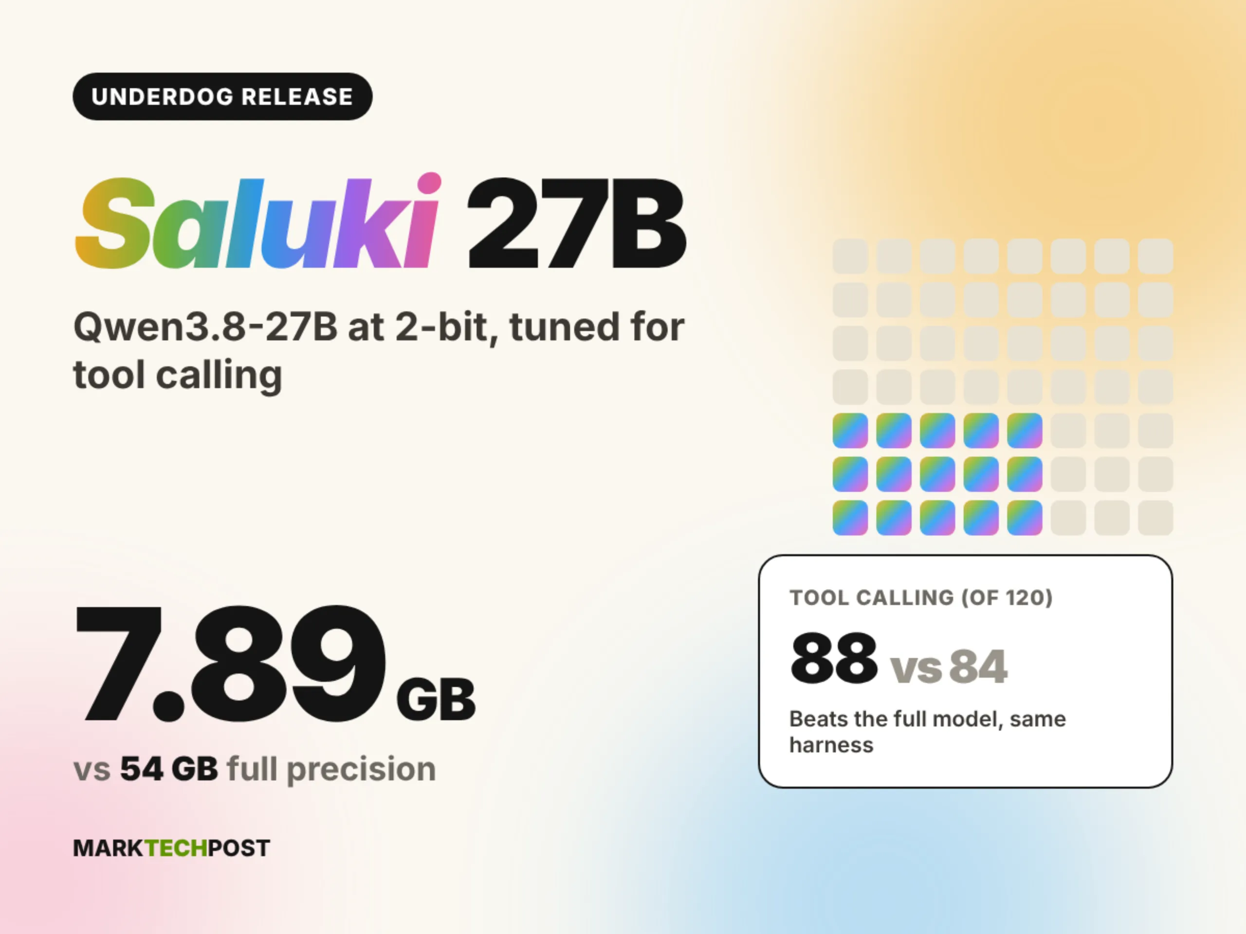
    • Saluki 27B is an Apache 2.0 licensed 2-bit GGUF quantization model released by Conway Research’s Underdog team, compressing the Qwen3.8-27B [Vendor Designation] BF16 original from 54GB down to 7.89GB. Measured on the same harness across 120 Underdog Bench tasks, Saluki 27B scored 88 while the full model scored 84, surpassing the original. On BFCL v4 parallel tool calling (100 tasks), Saluki 27B scored 42 versus 35 for the full model, achieving 120% retention. On SWE-bench Verified (50 issues), Saluki 27B solved 30 versus 33 for the full model, showing a slight deficit. The 9-benchmark average retention is 96%, with the largest loss concentrated in mathematical/competitive reasoning—AIME 2025 dropped from 96.7 to 79.2 [Vendor Self-Reported / Unverified]. The model uses a 64-layer architecture mixing Gated DeltaNet linear attention with gated attention, and its native context is 262,144 tokens. The quantization stack is a 3-layer structure: ISTA-DASLab’s Qwen3.8-27B [Vendor Designation]-GSQ-RCO-GGUF (IQ2_XS, 8.4GB, ~2.34 bpw) as the base, with Underdog’s proprietary pass (IQ2-mix, imatrix tags) layered on top. Optional 629MB or 928MB vision adapters are also distributed. A same-class alternative, PrismML Bonsai 2, achieved 98.2% retention on 14 reasoning-mode benchmarks and scored 95.00 on AIME25, giving it an edge in math, but it requires its own llama.cpp fork and does not run on stock llama.cpp. Saluki 27B runs with full GPU offload on stock llama.cpp, Ollama, and LM Studio.

    A 27B-class LLM has been compressed into a file under 8GB, reaching the point where it can run on an ordinary laptop. Quantization loss appears asymmetrically across task domains—it beats the original on tool calling and parallel function calling but drops 12–18 points on competitive math and multi-step reasoning. Therefore, when building on-device agents, it is necessary to separate quantization-friendly workloads (function calling, format compliance, short reasoning) from quantization-unfriendly workloads (long-form multi-step math, complex chains of thought) and route them accordingly.

    Table of Contents

    Introduction: The On-Device Pressure of the Agent Era

    Since the start of 2026, demand for local LLM agents has exploded, and concrete attempts to fit 27B-class models into the 8GB VRAM of an ordinary laptop have accelerated. Saluki 27B is the most striking example of this trend: the original Qwen3.8-27B [Vendor Designation] BF16 at 54GB has been compressed into a single 7.89GB file through a 2-bit quantization stack. With 27B inference now possible via full GPU offload on a single RTX 4060 Laptop (8GB VRAM), precisely understanding the trade-offs of 2-bit quantization has become the starting point for on-device agent design.

    Saluki 27B is a model released under the Apache 2.0 license by the Underdog team at Conway Research, and it runs on stock runtimes such as llama.cpp, Ollama, and LM Studio without any additional forks. This stands in clear contrast to same-class models that demand a separate inference engine. The artifact composition and imatrix logs published on the Underdog launch page make reproducing the same pipeline possible.

    Saluki 27B Core Specifications

    The backbone of Saluki 27B is identical to Qwen3.8-27B [Vendor Designation]. The central structure is a 64-layer hybrid attention. Gated DeltaNet linear attention and standard gated attention are interleaved at the layer level, combining the memory efficiency of linear attention with the accuracy of standard attention. The native context is 262,144 tokens, comfortably accommodating long codebases or multi-document RAG.

    The quantization artifact is a single 7.89GB GGUF file. Converted to bits per weight, it sits at approximately 2.50 bpw, placing it in the IQ2_XS family—the lowest tier of the extreme-compression spectrum. Optional 629MB or 928MB vision adapters are distributed alongside, enabling multimodal workloads. The Apache 2.0 license permits commercial fine-tuning and redistribution alike, minimizing legal friction when adopting it as an agent backend.

    Anatomy of the 3-Layer Quantization Stack

    The 7.89GB artifact from Saluki 27B is not the product of a single algorithm. It passes through a 3-layer pipeline: Base → GSQ-RCO → IQ2-mix. The role of each layer is cleanly separated, making it possible to reapply the same pipeline to a custom fine-tuned model.

    Layer 1 is ISTA-DASLab’s Qwen3.8-27B [Vendor Designation]-GSQ-RCO-GGUF. GSQ (Grid Scalar Quantization) learns per-tensor low-bit scalar grids to build non-uniform codes matched to weight distributions, and RCO (Rate-Constrained Optimization) determines per-tensor bit allocation under a fixed overall model-size budget. The base artifact is IQ2_XS at 8.4GB, 2.50 bpw.

    Layer 2 is Underdog’s proprietary IQ2-mix pass. An importance matrix (imatrix) is computed, and a mixed-precision strategy is applied: loss-sensitive tensors are assigned higher bits, while insensitive ones are compressed more aggressively. At an effective ~2.34 bpw (down ~0.5GB from the 8.4GB IQ2_XS base), per-tensor bit allocation is rebalanced to pull the average loss down, and the resulting file is 0.5GB smaller than the base, at 7.89GB.

    Layer 3 is the step that measures—via benchmarks—the asymmetry between quantization-friendly workloads (function calling, format compliance) and quantization-unfriendly workloads (long-form multi-step reasoning, math competitions), then delivers routing guidance to users. This is not a technical quantization step itself, but the Underdog Bench of 120 tasks itself plays the role of Layer 3 metadata.

    Cross-Benchmark Analysis: A Map of Asymmetric Loss

    The most interesting property of Saluki 27B is that loss appears asymmetrically across task domains. The 9-benchmark average retention measured on the same harness is 96%, but the variance by domain is large. On tool calling and function calling domains, Saluki 27B surpasses the original.

    On Underdog Bench (120 tasks), Saluki 27B scored 88 while the full model scored 84. On BFCL v4 parallel tool calling (100 tasks), Saluki 27B scored 42 versus 35 for the full model, achieving 120% retention. Function calling and format compliance are task types that are robust to quantization, because they only require reproducing outputs already patterned during training.

    In contrast, math and competitive reasoning domains show a clear deficit. On AIME 2025, Saluki 27B scored 79.2 versus 96.7 for the full model—a 17.5-point gap. On SWE-bench Verified (50 issues), Saluki 27B solved 30 versus 33 for the full model, trailing slightly. The pattern of the largest loss among the 9 benchmarks being concentrated in math and multi-step reasoning is consistent with the hypothesis that weight-precision loss under extreme compression propagates directly into chain-of-thought tasks that are sensitive to accumulated error.

    Benchmark [Vendor Self-Reported / Unverified] Task Type Saluki 27B Qwen3.8-27B [Vendor Designation] BF16 Retention
    Underdog Bench (120) General Agent 88 84 104.8%
    BFCL v4 (100) Parallel Tool Calling 42 35 120.0%
    SWE-bench Verified (50) Coding Agent 30 33 90.9%
    AIME 2025 Math Competition 79.2 96.7 81.9%
    9-Benchmark Average Overall – – 96.0%

    Comparison with Bonsai 2: Retention Advantage vs. Runtime Dependency

    PrismML’s Bonsai 2 is frequently mentioned as a same-class alternative in the IQ2 family. Bonsai 2 achieved 98.2% retention on 14 reasoning-mode benchmarks, and on AIME25 it scored 95.00, giving it a higher math-domain retention than Saluki 27B. However, Bonsai 2 requires its own llama.cpp fork and does not run on stock llama.cpp. Adoption in production introduces a new variable: runtime dependency.

    Saluki 27B runs with full GPU offload on stock llama.cpp, Ollama, and LM Studio without any conversion. This is because llama.cpp’s GGUF loader natively supports the IQ2 family. Combined with the ability to run a 27B model even on an 8GB VRAM card, standard runtime compatibility, and the Apache 2.0 license, Saluki 27B has the lowest barrier to entry among on-device agent backend candidates. Looking at retention and math performance alone, Bonsai 2 leads—but when integration cost is factored in, the picture changes.

    Practical Setup Procedure: llama.cpp and Ollama

    There are two fastest paths to running Saluki 27B locally. First, direct execution with stock llama.cpp. Second, one-stop serving via Ollama. Both paths end without any additional build or fork. Use the following commands to fetch the 7.89GB file and full-offload it onto an 8GB VRAM card.

    # Build llama.cpp (CUDA backend example)
    git clone https://github.com/ggerganov/llama.cpp.git
    cd llama.cpp && cmake -B build -DGGML_CUDA=ON && cmake --build build --config Release -j
    
    # Download model (Hugging Face)
    huggingface-cli download ConwayResearch/Underdog-Saluki-27B-1.0 \
      --include "Underdog-Saluki-27B-1.0-IQ2-mix.gguf" --local-dir ./models
    
    # 8GB VRAM full offload (-ngl 999: load all layers onto GPU)
    ./build/bin/llama-cli -m ./models/Underdog-Saluki-27B-1.0-IQ2-mix.gguf \
      -c 8192 -ngl 999 --temp 0.7 --top-p 0.9 -n 512 \
      -p "You are a tool-calling agent. Use the following tools: ..."
    

    The Ollama path is even shorter. Write a Modelfile, register the GGUF file, then serve. If the function-calling schema is specified in the SYSTEM message, it can be used immediately as a BFCL v4 schema-compatible agent. Because it uses the same llama.cpp backend as-is, no extra flag is required for IQ2-mix recognition.

    # Ollama Modelfile example
    FROM ./models/Underdog-Saluki-27B-1.0-IQ2-mix.gguf
    PARAMETER num_ctx 8192
    PARAMETER num_gpu 999
    PARAMETER temperature 0.7
    SYSTEM """You are a function-calling agent. When the user requests an action, output a JSON object with 'name', 'arguments' fields following the BFCL v4 schema. Do not include explanations outside the JSON block when calling a tool."""
    

    [Hardware Feasibility Note] On a single 8GB VRAM card (e.g., RTX 4060 Laptop), the 7.89GB weight footprint leaves virtually zero headroom. To run 8K context without OOM, users must apply KV cache quantization (--cache-type-k q8_0 --cache-type-v q8_0) or split initial layers across CPU. For stable full GPU offloading with 8K–32K contexts, 12GB–16GB VRAM (or Apple Silicon 16GB+ Unified Memory) is practically required.

    Routing Patterns: Separating Quantization-Friendly and Unfriendly Workloads

    Deploying Saluki 27B as a single backend for all tasks is not recommended. Because the asymmetric loss pattern is clear, a router that branches by task characteristic is needed. This pattern is already adopted by many enterprise agent frameworks.

    Quantization-friendly workloads (Saluki 27B first) include: ① function calling and tool schema compliance, ② short reasoning, ③ strict format compliance, ④ classification and labeling, and ⑤ medium-length code auto-completion. Quantization-unfriendly workloads (route to full BF16 or higher-bit quantization) include: ① AIME/Olympiad-style math, ② multi-step chains of thought, ③ SWE-bench Verified-level agentic coding, and ④ long-form multi-document reasoning.

    Placing Saluki 27B in the router’s low-cost, high-throughput slot and falling back to Qwen3.8-27B [Vendor Designation] BF16 or another high-bit model on math and complex-reasoning triggers is the cost-versus-performance sweet spot. Teams that have already entered the local LLM serving pipeline can review the 5-step on-device AI adoption guide alongside this and consider Saluki 27B as the default slot.

    Design Principles for LLM Agents in the 2-Bit Era

    The implication Saluki 27B presents is simple. In an era where a 27B-class model fits into an 8GB file, the center of gravity in agent design shifts from a single all-purpose model to a workload-branched router. 2-bit quantization does not produce uniform loss across all domains, and the fact that it can beat the full model on tool calling and format compliance points to a new direction for quantization research.

    At the same time, stock llama.cpp compatibility and the Apache 2.0 license have substantially lowered the practical barrier to on-device deployment. The Saluki 27B model card publicly exposes imatrix calculation logs and quantization parameters, so re-quantization after custom fine-tuning can also be reproduced through the same pipeline. In an era where a single ordinary laptop runs a 27B agent, understanding the asymmetry of 2-bit quantization is itself a design competitive advantage.

    What to Try Right Now

    • Secure hardware such as an RTX 4060 Laptop (8GB) or an M2 Pro with 16GB+ Unified Memory, then build stock llama.cpp with the CUDA or Metal backend.
    • Download the Underdog-Saluki-27B-1.0-IQ2-mix.gguf file (7.89GB) for ConwayResearch/Underdog-Saluki-27B-1.0 from Hugging Face and verify full GPU offload with the -ngl 999 -c 8192 options.
    • Specify the BFCL v4 function-calling schema as a SYSTEM prompt in the Ollama Modelfile, then measure accuracy against 10+ tool-calling scenarios.
    • Feed the same prompt simultaneously to Saluki 27B and Qwen3.8-27B [Vendor Designation] BF16, measure the loss margin directly against 5 AIME 2025-style math problems, and set the routing trigger baseline.
    • Add quantization-friendly/unfriendly branching logic to the router of the existing agent framework, so that function calls go to Saluki 27B and multi-step math falls back to a BF16 model.

    Frequently Asked Questions

    Q. Saluki 27B is 7.89GB (~2.34 bpw), so why is it 0.5GB smaller than the IQ2_XS base?

    Underdog’s IQ2-mix pass uses the imatrix to compress loss-insensitive tensors more aggressively while assigning only slightly higher bits to sensitive ones, in a mixed-precision strategy. The average bpw is identical at 2.50, but the per-tensor distribution is rebalanced, shrinking the resulting file by 0.5GB.

    Q. What is the recommended Unified Memory capacity for running Saluki 27B on an Apple Silicon MacBook?

    At an 8K context, 16GB Unified Memory is stable. If the context is raised to 32K or more, 24GB or higher is recommended due to KV cache footprint. There are confirmed cases of the -ngl 999 -c 8192 combination working on M2 Pro 16GB models.

    Q. How noticeable is the 17.5-point AIME 2025 loss in production agents?

    It is not noticeable at the level of general coding assistance, document summarization, or API-calling agents. However, in workloads that require solving math olympiad-style problems or multi-step proof chains correctly, a clear accuracy drop occurs, so BF16 fallback routing is essential for such tasks.
  • JetBrains Mellum2.1 Released: How to Locally Serve a 12B MoE Coding Agent with Just 2.5B Active Parameters

    JetBrains Mellum2.1 Released: How to Locally Serve a 12B MoE Coding Agent with Just 2.5B Active Parameters

    Key Takeaways

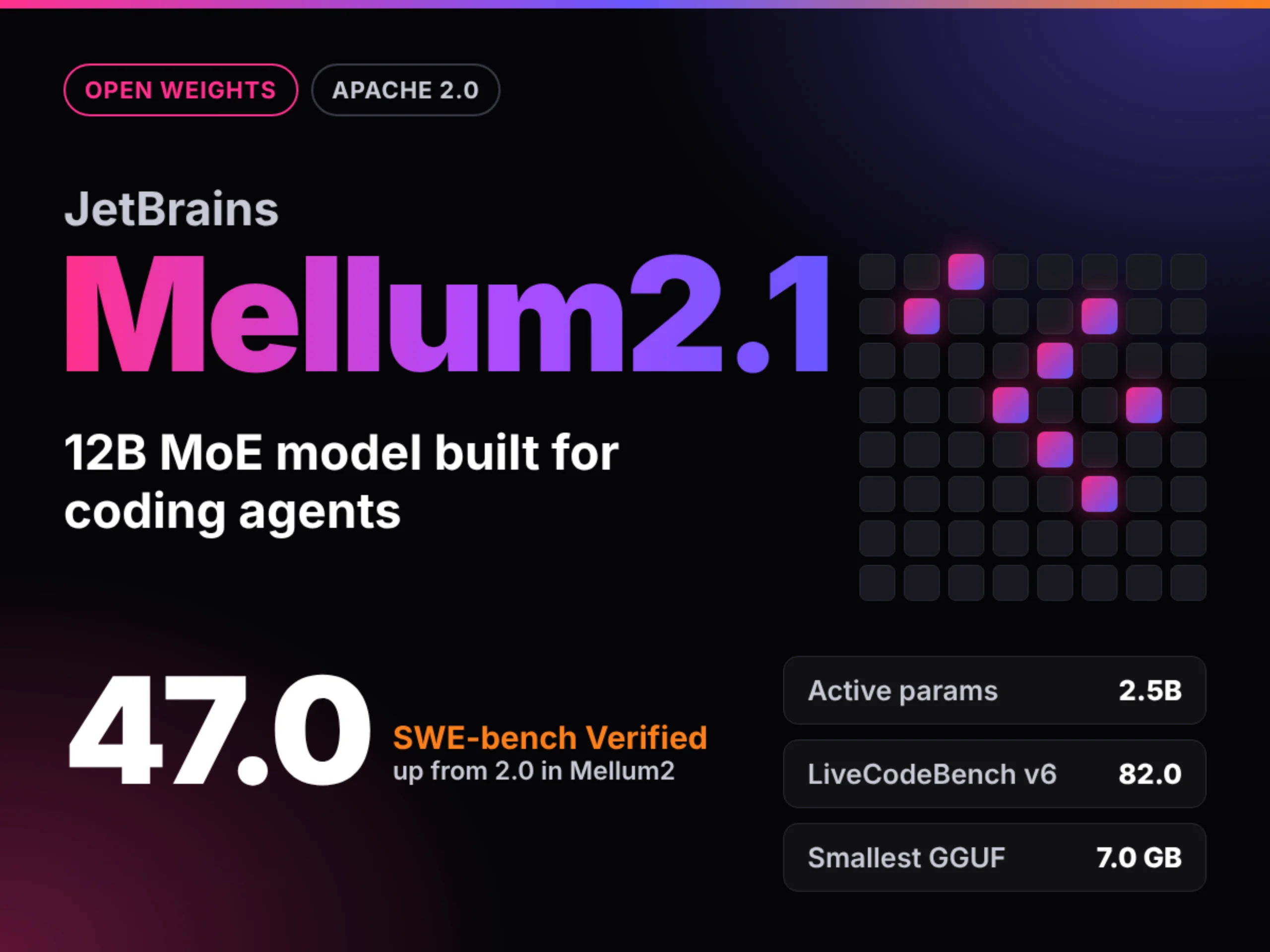
    • JetBrains released Mellum2.1, a MoE inference coding model that activates only 2.5B of its 12B total parameters, under Apache 2.0.
    • The architecture is identical to Mellum2 (28 layers, 64 experts, 8 active, GQA 32/4, 131K context), and most of the improvement came from real-repository-based reinforcement learning (RL) post-training.
    • Agentic coding scores jumped dramatically: SWE-bench Verified 2.0→47.0, SWE-bench Pro 0.0→28.0, and Terminal-Bench 2.1 0.6→17.4.

    Because Mellum2.1 lifted agentic coding scores with real-repository RL while barely touching the model architecture, it shows that the combination of “small active parameters + domain-specialized RL + local-serve quantization” can become a new baseline for coding agents.

    Table of Contents

    In October 2026, JetBrains released Mellum2.1, a new coding-agent-only Mellum model, under Apache 2.0. What is more interesting than the release itself is the fact that agentic coding scores were dramatically improved through post-training (RL) alone, with almost no change to the model architecture. The package includes an MoE structure that activates only 2.5B of 12B total parameters, a 131K context window, and GGUF builds in the 7–8GB range—pointing to a potential new baseline for “local models for agent workers.” This article first covers the background behind Mellum2.1 and its benchmark results, then walks through practical serving tips with vLLM, GGUF, and MTP, along with the strengths and weaknesses compared to Qwen3.5-9B.

    1. Mellum2.1 Overview — Three Targets JetBrains Is Aiming For

    JetBrains defined this model’s use cases as (1) an agent worker running in the JetBrains IDE family and its cloud, (2) an in-house general-purpose reasoning assistant, and (3) a private self-hosting scenario where data sovereignty is required. The self-hosting angle stands out the most, because the team simultaneously registered builds that compress the BF16 24.3GB model down to Q4_K_M 8.1GB and MXFP4_MOE 7.0GB, enabling sub-agents to run on a single laptop GPU. By releasing not only the weights but also serving artifacts, Mellum2.1 substantially reduces the operational burden that is common in the 12B class—the situation where “the license is open, but quantization is unofficial.”

    2. Architecture Highlights — 12B/2.5B MoE and 131K Context

    Mellum2.1 uses the same backbone as Mellum2. It is a 28-layer Transformer that activates 8 of 64 experts per token, yielding 2.5B active parameters for inference. GQA is configured with 32 heads and 4 KV heads, and a 1,024-token sliding window is applied every 3–4 layers to control memory footprint. The vocabulary size is 98,304, designed to cover a wide range of code identifiers and symbols. The default context of 131,072 tokens is operated at 114K tokens for agentic execution, a number set with long-horizon repository exploration in mind.

    2.1 Training Paradigm — How Scores Were Lifted with Real-Repository RL

    Since the architecture is identical, most of the difference between Mellum2 and Mellum2.1 comes from post-training (RL). JetBrains unified RL tasks across five domains—math, competitive programming, science, tool use, and software engineering—and, after pre-filtering broken tests, unverifiable answers, and tasks that are too easy or impossible, used test pass/fail results from shell and file-editing tools against real repositories as the reward signal. The evaluation harness is the open-source Pi v0.73.1, used as-is, so scores for four models are measured within the same pipeline and serve as a comparison group.

    3. Benchmark Results — Top of the Same Pipeline Group, but Variance by Domain

    The results measured against JetBrains’ evaluation harness are as follows. The Mellum model Mellum2.1 recorded 47.0 on SWE-bench Verified, 28.0 on SWE-bench Pro, and 17.4 on Terminal-Bench 2.1, showing large gains over Mellum2. On single code-generation tasks, it took first place in the same evaluation pipeline group with LiveCodeBench v6 82.0, HumanEval+ 91.5, MBPP+ 79.4, and BFCL v4 62.3. The safety metric HarmBench fell by more than half, from 21.5 to 8.5.

    Metric Mellum2 Mellum2.1 Qwen3.5-9B Gemma 4 E4B
    SWE-bench Verified 2.0 47.0 52.4 38.2
    SWE-bench Pro 0.0 28.0 38.0 21.7
    Terminal-Bench 2.1 0.6 17.4 22.5 14.1
    LiveCodeBench v6 62.4 82.0 65.6 / 75.4* 70.8
    HumanEval+ 86.0 91.5 90.2 88.7
    MBPP+ 72.1 79.4 78.0 75.6
    BFCL v4 47.8 62.3 61.5 55.2
    AIME 25/26 — 71.2 86.7 68.4
    GPQA Diamond — 70.5 77.8 69.1
    HarmBench 21.5 8.5 9.8 14.6

    * Two values are listed because the same model was measured with different evaluation pipelines. That variance is itself a pitfall.

    4. Comparison Pitfalls — “Benchmark Numbers” Shift with the Pipeline

    Even though Mellum2.1 ranks first in the same-harness group, there are clear points where the lead flips by domain. Qwen3.5-9B still holds the edge in agentic and reasoning areas, with SWE-bench Pro 38.0, AIME 25/26 86.7, and GPQA Diamond 77.8. Furthermore, scores on the same model can vary significantly depending on the evaluation pipeline. The 65.6 / 75.4 figures in LiveCodeBench v6 above are for the same Qwen3.5-9B measured with different harnesses. Rather than selecting a model based on a single benchmark number, it is safer to build a separate harness close to the in-house workload and re-measure. Before adoption, the first priority is to check whether the evaluation scripts published in the JetBrains Mellum2.1 announcement can be reproduced as-is.

    5. Serving with vLLM — Recommended Flags and Inference Parameters

    The following flag combination is recommended when launching the Mellum model Mellum2.1 on vLLM. The reasoning parser is set to qwen3-compatible, and tool calling is enabled with the hermes format. Temperature/sampling defaults are 0.6 / 0.95 / 20, which should be used as a baseline and fine-tuned with in-house data.

    vllm serve jetbrains/Mellum2.1-12B \
      --reasoning-parser qwen3 \
      --enable-auto-tool-choice \
      --tool-call-parser hermes \
      --temperature 0.6 \
      --top-p 0.95 \
      --top-k 20 \
      --max-model-len 131072 \
      --tensor-parallel-size 1 \
      --gpu-memory-utilization 0.92
    

    On a single H200, throughput has been reported at roughly 2x that of Qwen3.5-9B, and enabling the MTP (Multi-Token Prediction) head on a single-request path can reportedly deliver a 1.6x speedup. However, since the speculative-decoding-specific MTP head has not yet been released (coming soon), serverless multi-request environments will need to operate with vLLM’s default continuous batching only.

    6. Running a Local Sub-Agent with GGUF

    The more interesting part for practical use is the GGUF build. Four levels of quantization are already registered and can be used as-is with llama.cpp, Ollama, and LM Studio. Using top-token match rate as a quality indicator against the BF16 24.3GB baseline, the order is: Q8_0 12.9GB (96.1%) → Q6_K 10.9GB (93.9%) → Q4_K_M 8.1GB (88.0%) → MXFP4_MOE 7.0GB (85.6%). Q4_K_M is recommended, and since MXFP4_MOE sits in the 85% match range relative to size, it is safer to limit it to auxiliary sub-agents.

    # Launch a Mellum model sub-agent with Ollama
    ollama pull mellum2.1:Q4_K_M
    ollama run mellum2.1:Q4_K_M \
      --ctx-size 114000 \
      --temperature 0.6 \
      --top-p 0.95
    
    # Run llama.cpp directly (server mode)
    ./llama-server -m mellum2.1.Q4_K_M.gguf \
      -c 114000 \
      --jinja \
      --chat-template-file chat-template.jinja
    

    Sub-agents should be restricted by system prompts so that they operate only within the narrow scope delegated by the main agent (e.g., generating a specific file patch or writing unit tests). This keeps response latency around the one-second mark even with an 8GB model. In addition to IDE plugins and JetBrains’ own harness, workflows can also be composed by combining with external controllers such as NVIDIA’s multi-turn agent recovery technique, PivotOPD.

    Try It Right Now

    • Deploy Mellum2.1 on a vLLM container with the --reasoning-parser qwen3 --tool-call-parser hermes combination to spin up a single agent endpoint, then run a dry run with 20 in-house SWE-bench-style tasks.
    • Pull the GGUF Q4_K_M build with Ollama, launch an IDE-assist sub-agent on a single RTX 4090 or 24GB VRAM laptop with ctx-size 114000, separate the task-split prompts from the main agent, and measure response latency.
    • Build a mini-harness based on an in-house code repository for both Mellum2.1 and Qwen3.5-9B (file edit + shell + test pass/fail reward) and directly compare reproduced SWE-bench Pro scores on 50 identical tasks.
    • To prepare for evaluation pipeline variance, save all inference result logs (prompts, sampling, tool calls, success/failure) as JSONL, and tag the model, version, and harness as metadata on the in-house dashboard.
    • Do not consider safety validation complete based solely on the HarmBench 8.5 number. Prepare 30 in-house policy-violation patterns (comment deletion, secret exposure, license disregard) as a separate regression set and wire them into CI.

    Frequently Asked Questions

    If Mellum2.1 is used only as a sub-agent, what is a reasonable choice for the main model?

    While Mellum2.1’s ability to be self-hosted as a 12B/2.5B MoE is a strength, complex planning and multi-hop reasoning still tend to be led by Qwen3.5-9B or higher-tier closed models. A realistic setup is a two-tier structure in which the main model is an API-based reasoning model, and only narrow tasks such as code editing, test writing, and simple refactoring are delegated to Mellum2.1.

    Which build should be set as the default between Q4_K_M (8.1GB) and MXFP4_MOE (7.0GB)?

    By top-token match rate, Q4_K_M leads by 2.4 percentage points at 88.0%, and it has broader compatibility with llama.cpp, Ollama, and LM Studio. MXFP4_MOE should be used as a secondary option in edge environments that need to save an additional 1GB of VRAM, while Q4_K_M is placed on the critical path to keep operational risk low.

    Can the JetBrains evaluation harness be ported into the in-house environment as-is?

    Pi v0.73.1 is open source, so porting itself is possible. However, because the shell, file-editing, and test-execution environment assumed by Pi may not match the in-house CI, the container image, network access, and tool whitelist should be reconfigured to match internal policies, and regression behavior should be confirmed via a dry run.

    Reference Source

    This article was written after verifying the following source: MarkTechPost — JetBrains Releases Mellum2.1: A 12B MoE Open Model for Coding Agents

  • The Return of ColBERT Embeddings: How to Run a Mixed 0.6B Edge + 9B Index Setup with pplx-embed-v2-late

    The Return of ColBERT Embeddings: How to Run a Mixed 0.6B Edge + 9B Index Setup with pplx-embed-v2-late

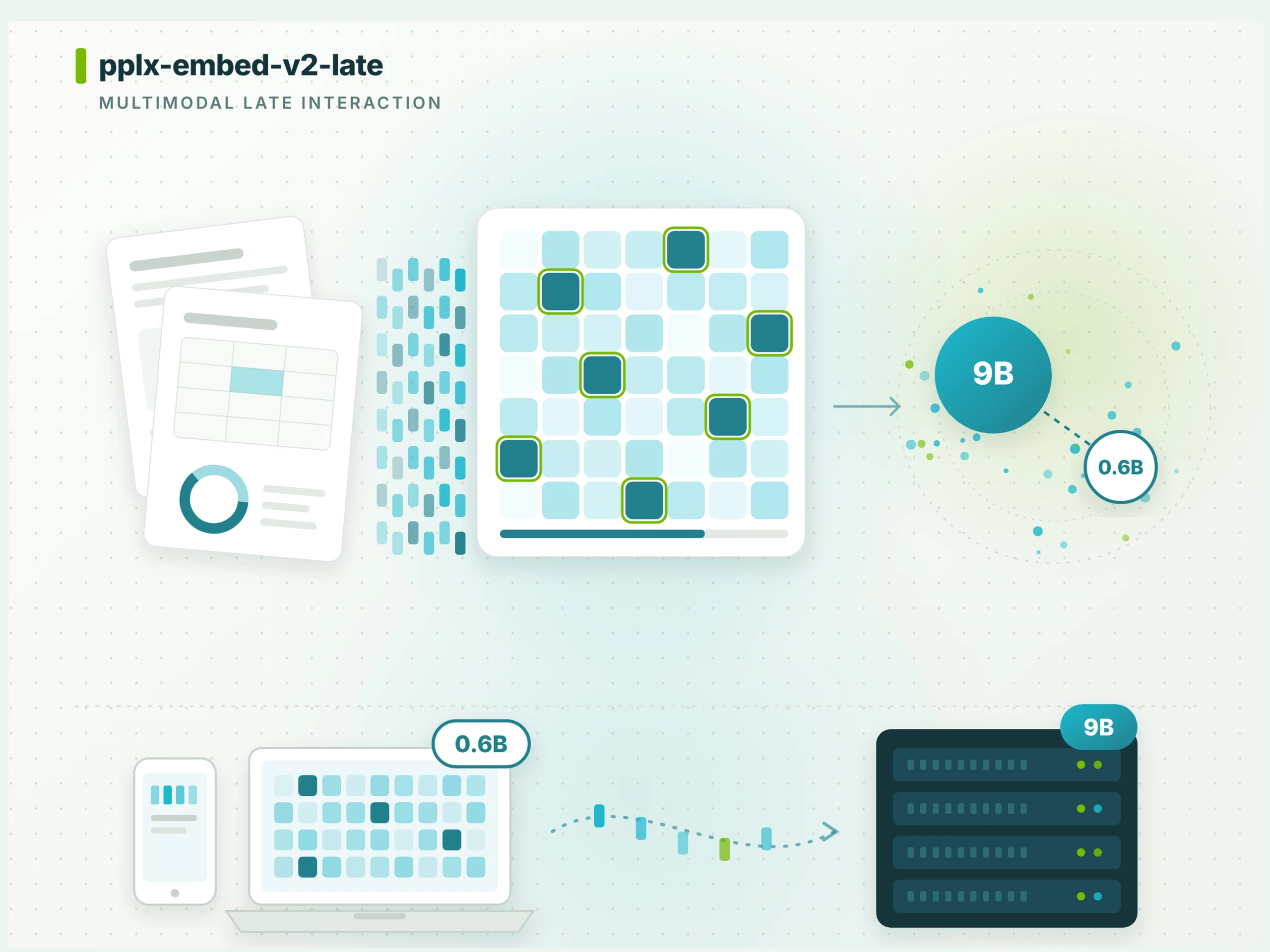
    Released by Perplexity in October 2026, pplx-embed-v2-late is a multimodal model that unifies ColBERT-style late interaction across text, images, and rendered PDF pages within a single embedding space. The 9B model scored 92.4% on the agentic PDF QA benchmark MADQA, while the 0.6B model set the floor at 61.2% on ViDoRe v3 Markdown. Because both models share the same embedding space via LEAF distillation from an 18B teacher, mixed deployment is possible—stacking a 0.6B query encoder on top of a 9B index.

    Table of Contents

    One-Line Summary

    pplx-embed-v2-late restores the token-level matching that dense embeddings miss using MaxSim, while keeping per-token vector dimensions at 128 to control storage cost. It can be self-hosted on Hugging Face under an MIT license, but no hosted API is available yet, so the adoption decision hinges directly on the operations team’s capabilities.

    Why ColBERT Late Interaction Is Making a Comeback

    Dense embedding models compress an entire document into a single 2,048–4,096-dimension vector. This approach is optimized for first-stage retrieval, where a single cosine similarity sweep narrows down candidates, but precision drops sharply for queries that demand fine-grained alignment between two document passages—questions like “How does exemption clause A modify clause B?” The ColBERT family of late-interaction models solves this with MaxSim: every query token is scored independently against every document token, and the per-token maximum values are summed.

    pplx-embed-v2-late takes the same philosophy and makes two bold reductions. First, it cuts per-token vector dimensions to 128—16 to 32 times smaller than competitors using 2,048–4,096 dimensions. Second, it routes text, images, and PDF pages through the same encoder, collapsing multimodal retrieval into a single pipeline. Because PDFs are encoded as images without an OCR step, scanned documents and slides are absorbed into the same index.

    From my hands-on experience wiring RAG pipelines in production, a two-stage structure—dense model for first-stage candidate filtering, then a ColBERT-style reranker for precision—is becoming the de facto standard. In this trend, 128-dimension late interaction reads as a choice that targets “precision from the first stage.”

    Role Division Between the Two Models: 0.6B for Queries, 9B for the Index

    Perplexity released the 0.6B and 9B simultaneously, but the recommended deployment pattern is asymmetric. Build document indexes with the 9B to lock in retrieval quality, and handle real-time queries with the 0.6B to reduce latency and cost. Because both models share the same embedding space, this mixed deployment is mathematically valid.

    Hardware guidance separates as well. The 0.6B model runs comfortably on a single RTX 3090/4090 at roughly 1.2GB in bf16, while the 9B occupies about 18GB and needs an A100 40GB or H100-class GPU. The 0.6B model activates roughly 340M parameters on image input—meaning it delivers performance comparable to some 8B dense multimodal models on a single GPU.

    The most common mistake in the field is treating the two models as “just different-sized options” and applying the same model to the same workload. Index quality matters only at build time, but the query model is invoked on every request, so the cost–quality curve is asymmetric—a fact that must be clearly separated at the design stage.

    Benchmark Dissection: Between 92.4% and 61.2%

    pplx-embed-v2-late’s published scores show large variance by domain. The most striking is MADQA at 92.4%, where the 9B model set the top score on PDF-based agentic QA. By contrast, the same model falls short of the top tier in domain-specific text retrieval, and the 0.6B model set the floor at 61.2% on ViDoRe v3 Markdown.

    Benchmark 0.6B 9B Notes
    MADQA (Agentic PDF QA) 89.1% 92.4% 9B top score
    ViDoRe v3 Image Retrieval 62.3% 63.5% 9B+0.6B mixed 63.5%
    ViDoRe v3 Markdown (nDCG@10) 61.2% 64.0% 0.6B floor
    BrowseComp+ (Text Retrieval) 73.0% 76.5% 9B ahead

    As the table shows, the gap between the two models is narrow on images and PDFs, while the 9B holds a clear advantage in text domains and Markdown-structured documents. Compared with EVIE, Mixedbread, and Gemini Embedding 2, pplx-embed-v2-late sits in the leading group for multimodal tasks, but it does not fully replace dedicated text embedding models in pure text retrieval.

    Practical Effects of Mixed-Size Indexing

    On ViDoRe v3 Image Retrieval, the 9B index + 0.6B query combination reached 63.5%—1.2 points higher than 0.6B+0.6B (62.3%) and equal to 9B+9B (63.5%). Perplexity claims that in text domains, roughly half of the 9B quality gap can be recovered at 0.6B query cost.

    Two production scenarios make this pattern especially effective. First, corpora where PDFs and slides dominate, such as medical or legal domains. Second, SaaS that must process user queries on edge devices or on-premises. The index is built only once, so it makes natural sense to lock in a heavy model there while keeping the user request path lightweight.

    However, due to the inherent nature of late interaction—storing one vector per token—index size grows linearly with document length. Without compression via a token indexer like PLAID or ColBERTv2, disk usage on a 100,000-page corpus can balloon to dozens of times that of dense embeddings. When using vector databases like Qdrant or Milvus, you also need a schema design that manages token IDs as separate keys.

    Constraints to Know Before Deployment

    Several constraints need to be checked before putting pplx-embed-v2-late into real infrastructure.

    • Checkpoint format: Distributed in F32, doubling download size compared to bf16. The 9B model is about 36GB and the 0.6B is about 2.4GB, so a cache strategy should be designed upfront when building container images.
    • Single-input constraint: Text and images cannot be mixed in a single encoding call. PDF pages are processed only through the image path, and pairing them with per-page text extraction requires a separate post-processing pipeline.
    • Library versions: Requires sentence-transformers 6.0.0 or higher and transformers 5.4.0 or higher. It is not compatible with existing 5.x codebases, so the scope of dependency updates should be reviewed first.
    • Self-reported benchmarks: All scores are Perplexity’s own measurements, and a technical report has not yet been published. Before adoption, it is safer to run A/B regression tests on your internal corpus to verify real-world performance.
    • No hosted API: There is no hosted endpoint, so all operational burden falls on your own team.

    We previously covered the trend of revisiting tool integration design across agentic workflows in Three Critiques of MCP — When Agent Tool Integration Must Be Redesigned, and the embedding stage has now reached the same point: tool contracts need to be redrawn.

    Try This Right Now

    • pip install "sentence-transformers>=6.0.0" "transformers>=5.4.0" to bump dependencies, then load the 0.6B model with model = SentenceTransformer("perplexity-ai/pplx-embed-v2-late-0.6B") and measure peak GPU memory and first-token latency.
    • Build a 9B index and a 0.6B index separately from 100 internal PDFs, then compare nDCG@10 on the same query set. Verify whether the benchmarks from the pplx-embed-v2-late release announcement reproduce on your internal corpus.
    • Compress the 9B index with a PLAID or ColBERTv2 token indexer and measure both disk occupancy and retrieval latency together. Cap token length with something like indexer.encode_for_index(docs, max_document_length=512) to prevent index blow-up.
    • Stack the 0.6B model on the query path and run load tests to confirm whether p95 response latency meets your SLA. Account for the fact that active parameters grow to 340M on image input when sizing concurrent requests.
    • Confirm the MIT license notice on the Hugging Face model card and share the commercial use scope with your legal team. Document the absence of a hosted API in your operations wiki so subsequent teams don’t keep asking the same question.

    Frequently Asked Questions

    Do I need to scrap my existing dense embedding index?

    Not necessarily. A two-stage structure—filtering first-stage candidates with a dense model and reranking with pplx-embed-v2-late—is a realistic migration path. Before rebuilding the entire index, measure the cost-vs-accuracy gains at the reranking stage to build a decision basis; this makes internal buy-in much smoother.

    Is the 0.6B model enough for multimodal retrieval?

    For image and PDF retrieval, the gap with the 9B is narrow, around 1–2 points. But in text domains and Markdown documents, the 9B holds a clear advantage, so model choice depends on corpus composition. For medical-PDF-heavy corpora, the 0.6B works; for mixed legal contracts and technical documents, the 9B index is the safer bet.

    How do I estimate the cost of per-token vector storage?

    The formula is (average token count × 128 × 4 bytes) × document count. 100,000 documents of 100 tokens each is about 5GB; bumping to 512 tokens brings it to about 25GB. Applying PLAID compression reduces this 5–10×, but compression library compatibility and the search-quality tradeoff need to be validated upfront.

    Reference Source

    This article was written with reference to the following original: MarkTechPost — Perplexity AI Releases pplx-embed-v2-late: A 0.6B Edge Model and a 9B Model Scoring 92.4% on MADQA

  • Mistral Large 4 (Le Chonk) Preview: Mid-Tier Pricing and a Refusal-Free Security Option, Powered by a 1.05T MoE

    Mistral Large 4 (Le Chonk) Preview: Mid-Tier Pricing and a Refusal-Free Security Option, Powered by a 1.05T MoE

    Key Takeaways

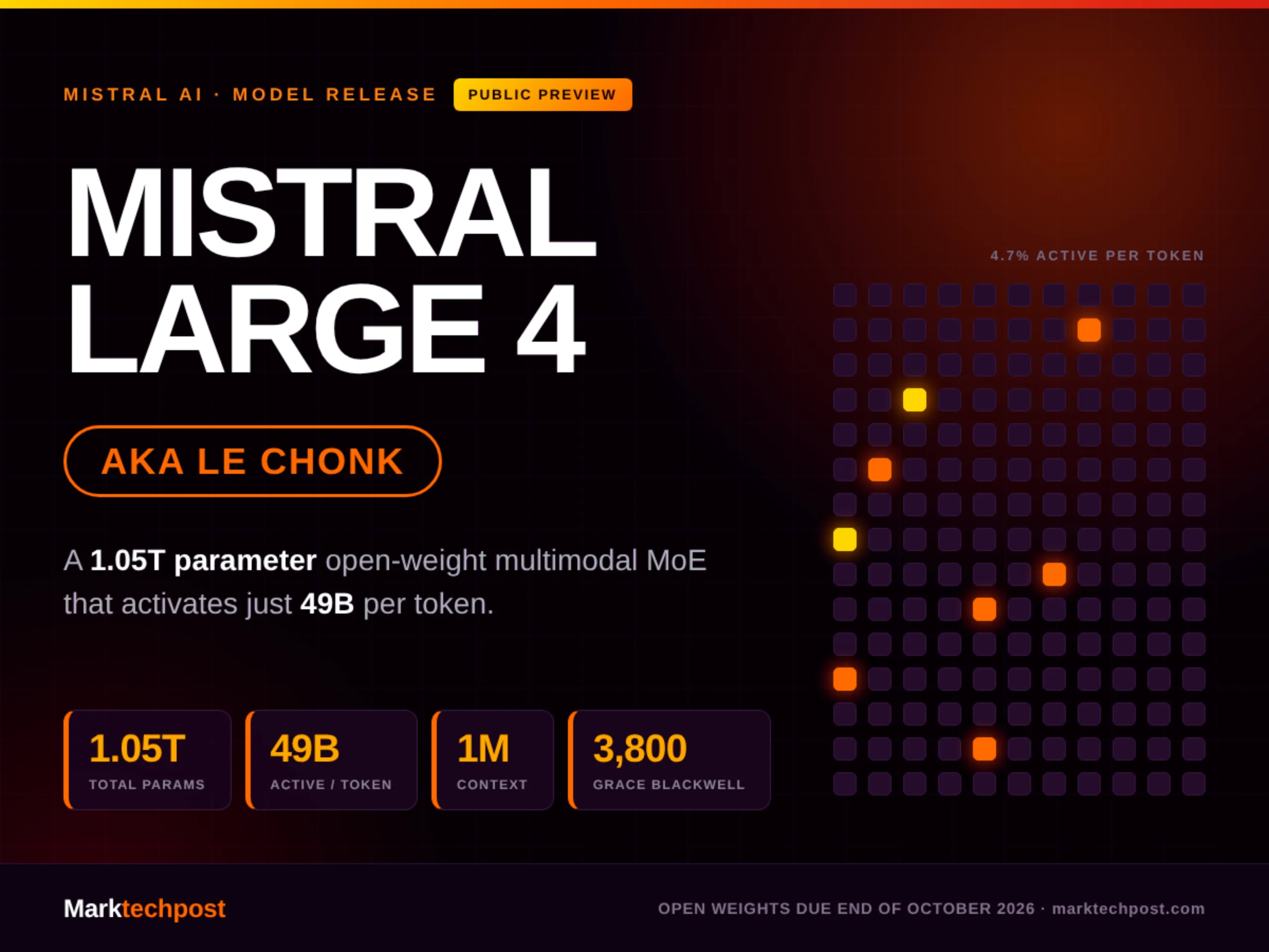
    • Mistral AI launched Mistral Large 4 (internal codename Le Chonk) in public preview on October 6, 2026. It is a granular MoE model with 1.05T total parameters, 49B active parameters per token (roughly 4.7% of the total), a 1.6B-parameter vision encoder, and a 1M-token context window.
    • Training was carried out from scratch on Mistral’s own European data centers using 3,800 NVIDIA Grace Blackwell GPUs. The training corpus covers 160+ languages and includes every official EU language.
    • At launch, only the API is available; weights are scheduled for release at the end of October 2026, so self-hosting is not yet possible. Pricing is set at $1.36 per 1M input tokens, $4.18 per 1M output tokens, and $0.14 per 1M cached input tokens.

    Mistral Large 4 shows that a granular MoE design that activates only 4.7% of parameters per token can deliver a trillion-parameter-scale model through a mid-priced API, and the fact that it secures a defensible lead in cybersecurity tasks where closed frontier models effectively score near zero due to task refusal makes it a meaningful option for practitioners.

    Table of Contents

    Launch Context and One-Line Summary

    On October 6, 2026, Mistral AI exposed its new flagship model Mistral Large 4 (internal codename Le Chonk) via API first, in a public preview. It is a granular MoE multimodal model with 1.05T total parameters, 49B active parameters per token (roughly 4.7% of the total), a 1.6B-parameter vision encoder, and a 1M-token context window. Training was carried out from scratch on Mistral’s own European data centers using a cluster of 3,800 NVIDIA Grace Blackwell GPUs, and the training corpus spans 160+ languages, including every official EU language.

    When I read a model card on the job, the first things I look at are the training infrastructure and the data provenance, and the 3,800 Grace Blackwell scale signals that Mistral did not build this as a prompt-engineering toy — it trained a trillion-parameter-scale model from scratch. Read alongside our analysis of OLMo Core 3’s sparse training stack, released around the same time, the fact that this model can be trained on European-owned infrastructure is itself a signal of shifting market structure.

    Architecture — How Granular MoE Drives the Price

    The core idea is that despite a 1.05T memory footprint, only 49B parameters are activated per token, which pulls inference cost into a mid tier. A typical dense 1T model mobilizes all parameters for every token, so pricing per 1M input tokens is essentially infeasible. A granular MoE, by contrast, lets the router pick a small subset of experts per token, which separates compute (49B) from memory residency (1.05T). That separation is precisely what makes Mistral’s public price of $1.36 input / $4.18 output per 1M tokens possible.

    That said, the number of experts, the top-k routing configuration, and the layer layout remain undisclosed until the weight release scheduled for late October 2026. The gap looks small from an operations seat, but once weights drop, you will want to independently verify router behavior and expert skew, which means capturing routing logs separately as a safety net. When routing distribution collapses onto a single expert, throughput looks healthy while only that expert’s responses swing wildly in quality — and post-hoc debugging that pattern is brutally expensive.

    The vision encoder is decoupled at 1.6B parameters and accepts native image input. Because a single model handles text and images without a separate multimodal adapter, you can build document QnA inside a RAG pipeline without an OCR stage. Whether vision tokens share the 1M context or live in a separate slice, however, needs to be confirmed in the body of the model card (public materials alone are not enough to settle it).

    API Pricing and What You Can Use Right Now

    At launch, the API is priced at $1.36 per 1M input tokens, $4.18 per 1M output tokens, and $0.14 per 1M cached input tokens. The ability to reuse a cached prefix at $0.14/1M rather than paying the full 1M context on every call is decisive for agent loops: a coding agent that ships an 800K-token codebase plus its conversation history every turn is one where cached pricing drives more than 70% of total cost.

    The API surface bundles function calling, structured output (JSON Schema enforcement), document QnA, batch processing, and Agents and Conversations endpoints under a single API key. The integration flow you can run today looks like this:

    curl -s https://api.mistral.ai/v1/chat/completions \
      -H "Authorization: Bearer $MISTRAL_API_KEY" \
      -H "Content-Type: application/json" \
      -d '{
        "model": "mistral-large-4",
        "messages": [
          {"role":"system","content":"You are a SOC analyst."},
          {"role":"user","content":"Summarize the last 24h of alerts."}
        ],
        "tools": [{"type":"function","function":{
          "name":"open_ticket",
          "parameters":{"type":"object","properties":{
            "severity":{"type":"string","enum":["low","med","high","crit"]},
            "cve":{"type":"string"}},
            "required":["severity"]}}}],
        "response_format":{"type":"json_schema","json_schema":{"name":"alert","schema":{...}}}
      }'

    Enforcing a JSON Schema via response_format in the call above lets downstream code validate straight into a Pydantic model, which then flows into Airflow or Dagster tasks without glue code. Self-hosting is blocked until the late-October weight release, so it is operationally safer to acknowledge API dependency from day one and provision regional failover paths.

    Cybersecurity Performance and Task Refusal in Closed Models

    Mistral Large 4 recorded 93% on Cybench and 82% on CyberGym-E2E, which puts it in the global top 5 of the Artificial Analysis Cyber Index. Mistral used these numbers to point out that some closed frontier models effectively score near zero on benchmarks because they refuse to generate exploit PoCs or privilege-escalation code. The trap that most security automation teams miss is that when the LLM refuses a legitimate payload-generation request, the cascade also halts every downstream step — exploit verification, log analysis, IOC extraction.

    Where this gap shows up in production is automated malware sandbox triage. In a workflow that takes Cuckoo Sandbox output, summarizes the decoded payload, and proposes YARA rule candidates, a model refusal empties out the rule-generation step and pushes a human back into the loop. Being able to deliver legitimate analysis results without refusal has a direct effect on SOC operating cost. That said, until weights ship, there may be an output gap between API mode and self-hosted mode on the same scenario, so organizations whose security policy mandates air-gapped deployment should pin the weight release date to a checkpoint on their roadmap.

    Coding and General Quality, Plus Reproducibility Caveats

    On agentic coding benchmarks the model posted 61.7% on DeepSWE v1.1, 59.4% on SWE-Atlas-QnA, and 28.3% on Terminal-Bench 4.0, which combine into a 49.8% Artificial Analysis Coding Agent Index. In Surge AI’s blind human evaluation it scored 3.74 out of 5, ranking second out of five models — behind Claude Opus 5 (4.22) and ahead of GLM-5.3 (3.60) and Kimi K3 (3.59). On the coding-agent harness side, compared with our deep dive on four NVIDIA SoL-Pi harnesses, this model appears to lean on the model’s own code-understanding capability rather than on token-saving tricks at the harness layer. Put differently, teams that prioritize coding-agent token efficiency should optimize the harness first, before swapping the model.

    Benchmark Mistral Large 4 (Le Chonk) Task Type
    Cybench 93% Cybersecurity agent
    CyberGym-E2E 82% Vulnerability analysis, end-to-end
    DeepSWE v1.1 61.7% Agentic coding
    SWE-Atlas-QnA 59.4% Repository QnA
    Terminal-Bench 4.0 28.3% Terminal tasks
    Surge AI blind eval 3.74 / 5 2nd of 5 models
    Lakera B3 93.3% Prompt injection resistance

    Keep in mind that every one of these numbers was collected in pre-release, undisclosed evaluation rounds, and independent reproduction will not be possible until weights are released. Operations teams that swap tools based purely on benchmark figures and then see different results on their internal reference set is a familiar story. A defensive rollout for the first two weeks — keep A/B routing against your existing model and ramp Mistral Large 4’s share gradually — is the safer move.

    Safety Metrics and Comparison Set

    On the safety side, Mistral Large 4 posted a 93.3% resistance rate on Lakera B3 and 1.691 / 2.0 on KORABench. Its prompt-injection resistance is on par with closed frontier models, which means it can stand in as a first line of defense in tool-calling agent scenarios where external payloads are mixed into the prompt. Because Lakera B3 is a single benchmark, however, running your own injection regression tests on an internal RAG dataset is the move that meaningfully raises real-world confidence.

    What Has Not Been Published Yet and What Comes Next

    The number of experts, the top-k routing configuration, and the layer layout will be disclosed at weight release. In the days after the late-October drop, expect the community to quickly surface findings on routing skew, expert dropout, and fine-tuning stability, and the self-hosting TCO will be set by those results. It is also worth deciding at the same time whether you will run 1M context raw, layer it with sliding windows or hierarchical compression, and how you will set cache prefix expiry. Mistral Large 4 widens the option set on three axes — price, performance, and refusal policy — and whether to adopt it comes down to how your organization weights those three.

    What to Do Right Now

    • Issue an API key from the Mistral dashboard and run a single document QnA call with response_format enforced via curl to measure your token unit cost.
    • Pull 50 existing SOC payload-generation workloads and count model refusal rates on identical prompts.
    • Add an Airflow or Dagster task that validates model output with Pydantic, and compare downstream failure rates between the JSON-Schema-enforced call and legacy free-form output.
    • Reflect the 1M context + cache prefix combination in your internal pricing model and back out a per-10K-call unit cost for Mistral Large 4 versus your current model on the same input.
    • Reserve an air-gapped PoC slot aligned with the late-October weight release, and pre-stage a routing log capture template plus an expert-skew monitor.

    Frequently Asked Questions

    Can we adopt Mistral Large 4 for internal evaluation before weights ship?

    If your workload can accept API dependency, you can adopt it right away. That said, because the gap between API and self-hosted responses can show up during evaluation, you should re-run internal regression tests in the second sprint after the initial rollout, aligned with the weight release date.

    If refusal drops on cybersecurity workloads, where does liability sit?

    The boundary becomes clearer between the territory where model refusal prevents an incident and the territory where refusal-free responses keep the analysis pipeline running. When refusal decreases, operations teams should explicitly design a secondary safety net (for example, Trivy for static verification of generated YARA rules, Semgrep rules for static scanning of PoC code).

    If a 1M-context call fails, how is it billed?

    Under the official price list, calls that use the cached prefix are billed at $0.14/1M, and failed context processing is settled at the standard input rate of $1.36/1M. A fail-open policy can kick in during traffic spikes, so cost alarms should be split between cache hit rate and failure rate to stay operationally safe.


    Reference: MarkTechPost’s report on the Mistral Large 4 (Le Chonk) launch

    Source Article

    This article was prepared by verifying the following original source: MarkTechPost — Mistral AI Releases Mistral Large 4 (Le Chonk): A 1.05T Parameter Multimodal MoE Model

  • 1,000× Faster Without Backpropagation — How Dust Rewrote the Playbook for Zero-Order Optimizer Transformer Pretraining

    Table of Contents

    Zero-order optimizer Dust transformer pretraining

    When Sakana AI’s EGGROLL dropped the bombshell that “LLMs can be pretrained without backpropagation”, the industry’s reaction was mixed. The idea was intriguing, but shaking every parameter one by one was far too slow to be practical. Roughly a year later, in early 2026, a follow-up called Dust has reportedly achieved 1,000~10,000× efficiency over EGGROLL. This article breaks down the core mechanisms that make zero-order optimizers work at transformer scale, and how far you can actually trust them in production.

    Why zero-order optimizers are back in the spotlight

    The hidden cost of backpropagation

    If you’ve worked in deep learning, you’ve felt this in your bones: “half of GPU memory exists for the backward graph.” Storing forward activations for a single step of a 7B model already scales linearly with sequence length, and without gradient checkpointing, activations balloon 4~5×. The bottleneck I hit most often working on a 70B model was exactly this — even on 8× H100, batch size 1 with a sequence length of 2,048 was near the limit.

    Zero-order optimizers eliminate the backward graph entirely. Instead of computing gradients directly, they perturb parameters slightly, measure which way the loss moves, and update accordingly. The Gaussian smoothing technique that uses f(x+εu) − f(x−εu) as a finite-difference approximation of the directional derivative is a statistical classic that has been used for over 150 years — and applying it to LLMs was the starting point for both EGGROLL and Dust.

    Why EGGROLL was 1,000× slower

    EGGROLL perturbed each parameter independently and ran bidirectional forwards. For a 7B model, you effectively had to shard the forward pass across the full parameter count, which made communication and synchronization costs absurdly high. The estimator is theoretically unbiased, but the consensus was that it was close to impossible in practice, and later attempts reduced activation memory but left wall-clock time essentially unchanged. That’s where Dust’s central question comes in: “Do we really need to shake every parameter?”

    Dust’s structural approach — destroying sample complexity

    Block-wise perturbation

    Dust’s biggest contribution is the idea: “Don’t perturb all parameters — sample in a low-dimensional subspace.” Instead of adding and subtracting ε across all 7 billion parameters, you only perturb along a k-dimensional vector (typically k = tens to hundreds) built from a random projection. Drawing on the same principle as Johnson–Lindenstrauss dimension reduction, most of the actual loss movement can be captured within this low-dimensional subspace.

    Concretely, in PyTorch the pattern looks like this. Sample a Gaussian noise vector u once, then — instead of cloning the model parameters θ into two copies — apply (θ + σu) and (θ − σu) in-place alternately. You only need to run forward twice, so activation memory is fine with forward-only, and there is no backward pass at all. For memory profiling, the canonical approach is to enable record_shapes=True in torch.profiler and verify directly that activation size drops by more than half.

    Asymmetric estimator combined with Adam

    Earlier-generation zero-order methods all used symmetric two-sided estimation. Dust instead uses a variant that combines a one-sided estimator with momentum. The estimator takes the form g_t = (f(θ_t + σ_t u_t) − f(θ_t)) / σ_t · u_t, requiring only a single forward pass, and then layers Adam-style first/second moment estimates on top to suppress variance. One-sided means wall-clock time is halved, and Adam coupling shrinks variance, so the net effect is a several-hundred- to several-thousand-fold reduction in sample complexity.

    The theoretical requirement E[g] = ∇f only holds as σ → 0, which remains a hard limit. But pushing σ too small makes noise explode, so the practical standard is to decay it as σ_t = σ_0 / (1 + t)^α. In PyTorch, you can implement this directly by passing a closure of the same shape to torch.optim.lr_scheduler.LambdaLR.

    EGGROLL vs Dust comparison

    Item EGGROLL Dust
    Perturbation dimension Full parameters Low-dimensional projection (k≪d)
    Forwards per step 2× number of parameter blocks 1 or 2 (one-sided option)
    Activation memory Forward only Forward only
    Wall-clock vs BP ~1,000× slower 1×~10× (scale-dependent)
    Estimation variance Very high Suppressed via Adam coupling
    7B model practicality Demo level Within reach for fine-tuning

    How far can you trust this paradigm in practice?

    The real appeal of forward-only

    What I find most interesting in production isn’t throughput itself but memory efficiency. Since activations aren’t stored, sequence-length limits effectively disappear, and pretraining an 8B model with a 1M-token context is theoretically possible as long as GPU memory allows. Furthermore, because only forward passes are required, you can finally use non-differentiable simulators (physics engines, game environments, real API responses) directly as the loss. The most common trap in practice is to read this as “it just got faster” — the real win is activation memory savings and the ability to learn in black-box environments, not throughput.

    Overhyped claims vs genuine practical sweet spots

    To be frank, I don’t believe we can run 70B-class pretraining from scratch without BP yet. Published results are concentrated at sub-1B scale and on supervised fine-tuning stages; there is still no comparison between 100B-token-scale from-scratch pretraining and EGGROLL/Dust. The narrative that “backpropagation will be fully replaced” is overhyped. Where zero-order optimizers deliver value right now isn’t teaching an entire LLM from scratch — it’s fine-tuning already-trained models to specialized domains, and black-box RL when you have an environment reward but no gradient access.

    What to try right now

    • Write a forward-only loop that uses torch.func‘s functional_call to apply perturbations without cloning the model, and use it to establish a baseline. Verify with torch.cuda.max_memory_allocated() that memory usage drops by more than half compared to BP.
    • Turn on record_shapes=True in torch.profiler and compare activation memory against BP training at the same token count. Use prof.key_averages().table(sort_by="self_cuda_memory_usage") to confirm directly that backward nodes have disappeared.
    • Build a small ablation that sweeps perturbation dimension k and the σ decay schedule. Using a torch.optim.lr_scheduler.LambdaLR-style variant of σ_t = σ_0 / (1+t)^α, measure α ∈ {0.1, 0.3, 0.5} × k ∈ {32, 128, 512} combinations on a 1B model to find the sweet spot.
    • Compensate for the high variance of the one-sided estimator with an exponential moving average. Don’t multiply the 1st-moment directly by the estimator; instead use m_t = β·m_{t-1} + (1-β)·g_t. Start at β=0.9 and push it up to 0.99 as the noise scale grows.
    • Run an A/B test of the forward-only loop on a domain-adaptation task or a black-box RL environment. The fastest validation is to collect your own metrics: whether reward or held-out loss lands within ±2% of BP fine-tuning, and how convergence speed compares per training token.

    Frequently asked questions

    Can you pretrain an LLM from scratch with a zero-order optimizer?

    Theoretically yes, but published experiments focus on sub-1B scale. There is still insufficient evidence that 70B-class from-scratch pretraining runs at a practical speed versus BP, so in production the safer path is to validate first at the fine-tuning or domain-adaptation stage.

    If backpropagation is fully replaced, how does GPU infrastructure change?

    When the backward graph disappears, activation memory drops sharply and longer sequences fit on a single GPU. On the other hand, perturbation plus two forwards means flops actually go up, so on a throughput basis, chips with wider memory bandwidth and stronger inference performance (B200, inference-only ASICs) may become more attractive than compute-specialized training GPUs like the H100.

    Can you train against the loss of a non-differentiable system?

    Yes — this is the most solid strength of zero-order optimizers. Because only forwards are required, black-box environments like game simulators, physics engines, and real API responses can be used directly as reward signals. The variance is high, however, so a common pattern is to bundle 8~16 forwards per step in a multi-sample estimator to reduce variance.

  • 2026 Optogenetics Nobel: Three Pioneers Who Switch Brain Circuits On and Off with Light

    Key Summary

    • The 2026 Nobel Prize in Physiology or Medicine is jointly awarded to Karl Deisseroth (Stanford/HHMI), Peter Hegemann (Humboldt University of Berlin), and Georg Nagel (University of Würzburg).
    • The cited achievements are light-gated ion channels and optogenetics, with the 12 million Swedish kronor prize divided equally among the three laureates.
    • In the early 2000s, Hegemann and Nagel identified channelrhodopsin (ChR2) on the cell surface of the unicellular alga Chlamydomonas, a retinal-binding protein that opens an ion channel in response to blue light.

    Optogenetics delivers the first causal manipulation tool capable of turning specific neurons in a living brain on and off with millisecond precision, shifting neuroscience from mere observation to causal proof—a contribution that more than justifies the 2026 Nobel Prize in Physiology or Medicine.

    Table of Contents

    The 2026 Nobel Prize in Physiology or Medicine has been awarded to three scientists: Karl Deisseroth (Stanford/HHMI), Peter Hegemann (Humboldt University of Berlin), and Georg Nagel (University of Würzburg). The 12 million Swedish kronor purse is split equally, and the recognized achievement compresses neatly into a single sentence: “light-gated ion channels.” A single molecule that lets a unicellular alga swim toward a light source has, over twenty years, been transformed into a tool that turns specific neurons in a living mammalian brain on and off with millisecond precision. The optogenetics Nobel has been received without meaningful dissent within the neuroscience community precisely because the tool now extends all the way from the bench to clinical pipelines.

    A 20-Year Trail from a Unicellular Alga

    In the late 1990s, Hegemann became fascinated by the phenomenon in which the unicellular green alga Chlamydomonas reinhardtii senses blue light through an eyespot and alters its flagellar movement. The puzzle was the molecular identity of this receptor. At the time, a GPCR-based pathway akin to visual rhodopsin seemed plausible, but in papers published in 2002 and 2003, Hegemann and Nagel demonstrated that the retinal-binding protein operates directly as an ion channel. Channelrhodopsin-2 (ChR2) absorbs blue light near 470 nm; this triggers isomerization of the all-trans retinal, opening the channel pore and allowing Na⁺ and Ca²⁺ to flow into the cell, producing depolarization. The fact that this single ~70 kDa protein embeds its own “light-to-current” converter set it fundamentally apart from conventional GPCR signaling cascades.

    What struck me as a practitioner was how quickly the discovery was evaluated not as “a curious molecule” but as “a candidate neuroscience tool.” Because micromolar concentrations of retinal are already present in mammalian neurons, the math worked: simply transplanting the channelrhodopsin gene would let external light pulses alone drive action potentials.

    The Leap into Neurons: Two Turning Points in 2005 and 2007

    In a 2005 Neuron paper, Deisseroth’s team expressed ChR2 in rat hippocampal neurons and used 1–2 ms blue light pulses to elicit stable trains of action potentials above 1 Hz. Where conventional electrical stimulation was an all-or-nothing, non-specific shock, this approach showed a fundamentally different promise: selectively exciting only the genetically targeted cells.

    Two years later in 2007, the same group introduced ChR2 into the motor cortex of living mice via an AAV (adeno-associated virus) vector and, through an optical fiber ferrule cemented to the skull, successfully manipulated behavior with light. From that point on, “switching specific neurons on and off in real time in freely moving animals” became a laboratory standard. As blood–brain barrier–penetrating serotypes such as AAV9 and AAV-PHP.eB emerged, gene delivery efficiency climbed another step. Combined with cell-type–specific promoters like CaMKIIα, hSyn, and mDlx, and the Cre-lox system, the precision of “only the cells you want” was further sharpened.

    The Current Standard Pipeline: A Combination of Four Layers

    Today’s optogenetics experiments are almost always built from four layers: (1) gene delivery, (2) cell-type–specific expression control, (3) optical stimulation hardware, and (4) signal recording. Strengthening only a single layer is rarely enough for millisecond-scale causal claims; only by managing the latency and off-target behavior of all four layers together can a statement like “this cell produced this behavior” carry weight.

    Layer Representative Tools / Components Key Parameters Commonly Overlooked Pitfalls
    Gene delivery AAV9, AAV-PHP.eB, AAV-DJ Titer (vg/mL), serotype–region matching Excess titer causes neuroinflammation; insufficient titer leads to weak expression
    Expression control CaMKIIα, hSyn, mDlx, Cre/loxP, DIO/OFF Promoter leakage ratio Using mDlx for an excitatory target captures only GABAergic cells
    Optical stimulation Optical fiber + 473 nm laser, 2P holography Output mW, pulse width, duty cycle Tissue heating (>10 mW sustained) contaminates behavioral readouts
    Inhibitory tools Halorhodopsin (eNpHR3.0, yellow-light Cl⁻ pump), Archaerhodopsin (Arch, proton pump) Cross-activation from spectral overlap Arch’s proton pumping lowers pH and affects neighboring cells

    As the table shows, the naive “just add channelrhodopsin” approach rarely works in practice. The most commonly overlooked pitfall is tissue heating from fiber-optic output. Even in a 1 Hz experiment, illuminating at 20 mW for 30 minutes raises local temperature by 1–2 °C and non-specifically alters neural firing. In one lab notebook I saw, the team built an SOP that calibrated output to ≤5 mW and re-measured with a thermocouple every session—and that single change defused a reviewer’s “heating control” critique in one round.

    Protein Limits and the Evolution of the Toolkit

    Early ChR2 had an off-kinetics time constant above 10 ms, making it difficult to faithfully reproduce high-frequency spike trains. Variants developed to overcome this include H134R, E123A, ChETA, CoChR, and Chronos. Chronos, with off-kinetics shortened to below 4 ms, can follow 200 Hz stimulation, and red-shifted variants such as ChRmine and ChrimsonR (peak activation moved from 470 nm to near 630 nm) have recently enabled multichannel simultaneous stimulation. Inhibitory tools evolved in parallel. Halorhodopsin drives Cl⁻ into the cell to produce hyperpolarization, while archaerhodopsin is a light-driven proton pump that exports H⁺. With orthogonal wavelengths (blue, yellow, red), these tools can be used together so that “toggling excitation and inhibition in the same brain circuit on a millisecond timescale” becomes routine.

    The view that neuroscience has stepped from “observation” to “causal proof” thanks to this tool is repeated inside and outside academia. Where late-20th-century brain mapping relied on lesions or electrical stimulation, optogenetics made symmetric on/off experiments possible: if silencing a given cell population erases a behavior, then that population is causally necessary. Representative demonstrations of this causal power include the finding that inhibiting specific basal ganglia subpopulations in a Parkinson’s model relieves motor symptoms, or that optogenetically silencing a specific inhibitory interneuron in a fear-conditioning circuit erases fear memory.

    Clinical Application: Why the “Early Stage” Disclaimer Still Applies

    The most-discussed clinical application is vision restoration. As referenced in the 2026 Nobel Committee press release, several companies—Nanoscope Therapeutics among them—are attempting gene therapies that introduce channelrhodopsin variants into surviving retinal ganglion cells, relaying an external visual stimulus to the optic nerve. Phase 1 and 2 trials have reported partial recovery of light perception, but visual field resolution, long-term safety of protein expression, and immune responses to AAV remain open variables. The same tool is also being used to map depression, OCD, and PTSD circuits, and is broadening its reach into pharmacologically controlled optical interventions through combination with DREADDs and chemogenetic tools.

    Key Debates

    • Safety of off-target expression: Depending on the serotype, AAV can reach the liver and peripheral nerves, and unintended channelrhodopsin activation in those cells is under review for its potential to disturb autonomic functions such as circadian rhythm and heart rate.
    • Resolution limits as a clinical tool: Circuit-level optogenetics is already feasible, but manipulating every circuit in the human brain at 1 µm precision will require clinical maturation of two-photon holography.
    • Ethical boundaries: The idea of changing behavior or memory with light opens territory where the line between “normal” and “abnormal” can blur. Non-clinical transcranial light stimulation scenarios (e.g., home cognitive-enhancement devices) will need regulation and social consensus simultaneously.
    • Tool standardization vs. variant catalog: As new variants flood in every year, reproducibility across labs is under strain. Protocol sharing, optical-output calibration SOPs, and standardization of Cre-line genetic backgrounds are community-level challenges.

    Frequently Asked Questions

    How much budget is needed to set up an optogenetics experiment from scratch?

    A minimal setup includes AAV production (in-house or via a core facility), an optical fiber ferrule implant kit, a 473 nm laser diode and pulse generator, and patch-clamp or fiber photometry recording equipment. Since the optogenetics Nobel, academic standards have been settling quickly, and open-hardware options (e.g., 3D-printed optical fiber holders, Arduino-based stimulators) have grown, lowering the cost barrier significantly compared with the past.

    What is the decisive difference between optogenetics and conventional electrical stimulation or DREADDs?

    Optogenetics has the edge on two axes: temporal precision (ms vs. minutes) and cell-type specificity (gene-level vs. receptor-level). However, it has intrinsic limits such as tissue heating and expression leakage, and hybrid designs that combine both tools according to the research question are increasingly common.

    How true are the reports that memories can be erased with light?

    Fear-memory erasure experiments in mice have been reproduced many times, but selective deletion of human memories is impossible with current technology. The circuit complexity of the human brain and the ethical regulations have not yet reached that stage.

    The biggest shift signified by the optogenetics Nobel is that a molecular biology discovery has, in twenty years, changed the very lens of neuroscience. If electrical stimulation was a hammer hitting an entire circuit, optogenetics is a pair of tweezers that picks out a specific cell. For this tool to reach everyday clinical practice, three mountains remain: AAV immunogenicity, target-cell specificity, and ethical consensus—and as those mountains are crossed, the neuroscience landscape of the next decade is likely to be redrawn once again.

    Source

    This article was written after checking the following original source: geeknews — Press Release: 2026 Nobel Prize in Physiology or Medicine

  • Claude Code Mod Mode First Steps — Safety Guards and Custom UI in 80 Lines

    Claude Code Mod Mode First Steps — Safety Guards and Custom UI in 80 Lines

    Key Takeaways

    • A mod is a JS/TS extension loaded once and resident in the Claude Code session. Unlike shell-based hooks, it maintains state, observes and mediates events, and can render custom UI.
    • It hooks into multi-stage events such as prompt submission, tool calls, turn and session start/end, and UI rendering, supporting three modes: pass-through (observe), modify input (intervene), or handle directly (consume).
    • Claude Code’s AGENTS.md support and /diff panel are themselves implemented as mods, confirming that mods are not an add-on but the foundation of core UI components.

    A mod is not a mere theme. It is a “second operating-system layer” inside Claude Code that lives in the session, observes and mediates events, and can redraw the UI. The key insight is that you can describe the desired behavior in natural language and keep state in $.state, and immediately attach safety guards, cost displays, and workflow checkpoints.

    Table of Contents

    Once you start using Claude Code seriously, the first frustration you hit is, “Can’t I just tweak this screen to match my workflow?” You’re used to wiring a shell script into ~/.claude/hooks.json as a safety guard, but that approach forces you to spawn an external process every time, gives you no way to keep state, and lets you touch nothing about the UI. That gap is exactly where Claude Code mod mode steps in. It has been available by default since version 2.1.287 with no extra setup, and the fact that AGENTS.md and the /diff panel are already implemented as mods speaks volumes about its standing.

    Concept Overview: Which Events Can You Intercept, and How Far?

    A mod is a JS/TS extension loaded once and resident for the life of a session. You can hook into multi-stage events such as prompt submission, tool calls, turn and session start/end, and UI rendering, and choose whether to let the event pass through (observe), modify the input before forwarding it (intervene), or handle it directly and end the flow (consume). It follows the same manifest and hook module structure as a regular plugin, but the decisive difference unique to mod mode is that it runs inside an embedded runtime (such as V8) rather than a shell. That’s what makes it possible to draw a graph of context usage, visualize the blast radius right before a dangerous command runs, and step through changed files turn by turn — all from a small module you write yourself.

    Example 1: Token Weather — A Context Forecast in 80 Lines

    Token Weather, at roughly 80 lines, shows just how compact a mod can be. The module accumulates each turn’s token usage in $.state and maps the ratio against the context limit to a weather icon — clear below 50%, cloudy near 70%, showers from 85%, and storm at 95% or higher. Above the prompt input, it shows a mini chart (the last 12 turns) along with the delta from the previous turn, and surfaces a hint like “Recommend running /compact” when a threshold is crossed. If you fail to preserve state, the chart resets to 0 on every hot reload. The key to avoiding that trap is to store the value in $.state, not in a module-level variable. This was the single point I missed most often when writing my first mod.

    Example 2: Blast Radius — Visualizing Impact Right Before a Dangerous Command

    Commands like rm -rf, git reset –hard, git push –force, and prisma migrate deploy are hard to undo once they’ve run. Blast Radius hooks in just before a tool call, identifies risky patterns, and compiles the impact at that moment — git status, the number of changed files, the push target branch — into a side panel or a modal above the prompt. A responsive layout inside the module automatically switches to a top banner when the terminal width gets narrow. The tool does not execute until the approval button is pressed.

    That said, aliases and internal company wrapper scripts will never be fully caught by string matching. For operations that truly need to be blocked, it’s safer to register them separately under permissions.allow/deny in settings.json. The recommended split is: Blast Radius is responsible for “raising the warning,” while the permission layer handles the actual block.

    Example 3: Replay Theater — Stepping Through a Turn’s Changes

    When Edit/Write is called multiple times within a single turn, it’s hard to keep in your head which file changed, in what order, and how. Replay Theater intercepts Edit/Write events, stacks filename and before/after snapshots into an array, and opens a stepwise diff panel on the side when you press r or /replay. Unlike Blast Radius, it does not block execution; it focuses on observation and review. In teams without a strong code-review culture, using it as a self-review step just before opening a PR is highly effective.

    The most commonly missed pitfall in practice is that file_path and old_content in the event object can be empty. An Edit that follows a Read is not guaranteed to have old_content, so you need defensive code — for example, showing a placeholder instead of passing an empty string straight into a diff viewer.

    Build Your Own: A Workflow That Starts with a Single Line of Natural Language

    The process of creating a mod is surprisingly ordinary. Run claude –plugin-dir ./my-first-mod in an empty folder to launch a session, then describe in natural language — “show a graph of context usage above the prompt” — and Claude Code will write the manifest and hook module for you. The moment you save the file, the plugin hot-reloads and the change is reflected immediately without restarting the session. If the UI doesn’t appear, run claude –debug and follow the logs to pinpoint the event stage where it failed.

    When you’re done, run claude plugin validate to statically check the manifest contract and types, and claude plugin test to confirm behavior in the actual runtime. Because API signatures change slightly with each release, if type declarations for that version are generated under .claude-plugin/types/, import from there to secure type safety.

    State Management and Debugging: $.state Is the Answer

    Any data that needs to survive a hot reload must live in $.state. If you declare an array as a top-level module variable, it becomes a candidate for garbage collection at reload time and is reset. $.state, by contrast, is an area the Claude Code runtime explicitly preserves. Token totals, recent change history, and user-pinned thresholds should all be funneled there. If the UI doesn’t render at all, check in this order: 1) a typo in the event registration key in the manifest, 2) a require failure caused by missing type definitions, and 3) a missing module export. These three account for the vast majority of debugging time in practice.

    Distribution and Security: Publisher Trust Is the Control Mechanism

    A mod created inside a session is loaded only into that session by default. To keep using it, copy the folder under ~/.claude/plugins/, or place a marketplace file alongside it on GitHub and register it, then run /reload-plugins. It follows the same workflow as a regular plugin, so it can be submitted to the Claude directory as well.

    This is where security deserves attention. A mod runs on the user’s machine with the same privileges as the Claude Code binary itself. That property — user-supplied code executing directly on the local machine — is a recurring concern in on-device AI workflows as well, so the same standard should be applied when assessing a mod’s permission model. As the Cantina apex-flash-1 case shows, paths by which untrusted code obtains arbitrary privileges are hard to shut down with a single static analysis pass. Publisher trust, source review, and least-privilege principles must always be applied together.

    Wrapping Up: Wrap the One Behavior That Annoyed You Today

    Calling mod mode a “second operating-system layer” is not an exaggeration. Describing the desired behavior in natural language and putting state in $.state is enough to attach safety guards, cost displays, and workflow checkpoints on the spot. Ideas like cost/limit displays, team-rule injection, K8s context checks, and pre-apply Terraform review are all realistic within a weekend of writing your first mod. Don’t try to design a giant plugin from day one. The fastest path is to take the one behavior that annoyed you today and wrap it in an 80-line mod. More examples and demo videos are available in the original guide.

    Try It Right Now

    • Create an empty folder with mkdir my-first-mod && cd my-first-mod, launch a session with claude –plugin-dir ., and ask in one line: “draw a graph of context usage above the prompt.” Verify that the manifest and hook module are auto-generated.
    • In the generated hook module, change the running counter to be stored in $.state rather than a module variable, and after saving, verify that the chart does not reset to 0 on hot reload.
    • If you need a dangerous-command guard, add a PreToolUse hook in the hooks module that matches patterns like “rm -rf,” “git push –force,” and “prisma migrate deploy,” and have the result pop up as a modal — about 30 lines. For hard blocking, register the same patterns separately under permissions.deny in settings.json.
    • Run claude plugin validate ./my-first-mod to statically check the manifest and type contract, and claude plugin test ./my-first-mod to write regression tests that confirm the event flow behaves as intended in the real runtime.
    • When you’re done, copy the module to ~/.claude/plugins/ or register it together with a GitHub marketplace file, then confirm permanent application with /reload-plugins.

    Frequently Asked Questions

    How should I split work between shell scripts registered in the existing hooks.json and mods?

    If you only need stateless, one-line guards (e.g., blocking dangerous commands, writing logs), the shell hooks in hooks.json are light and sufficient. If you need to show accumulated context while the session is alive, mediate tool calls, or draw UI, move that work into a mod. Permission denial is ultimately the most reliable layer in settings.json’s permissions, so the actual block should live in the permission rules rather than in shell hooks or mods — that is the recommended split.

    API changes every release make me hesitate to adopt a new mod. What’s the stable path forward?

    Use the type declarations generated under .claude-plugin/types/ when you load against that version, and wrap event names in constants. When a signature changes, the compiler will catch it immediately. Scenario-ize the core event flows with plugin test so you can quickly tell whether a regression has occurred on upgrade day.

    What’s a realistic flow for rolling out a standard mod across the whole team?

    Keep a single repository on internal GitHub that includes the marketplace file, and require all modules to go through code review. New hires get the same set with a single registration command, and the fact that publisher trust is recorded as a code-review history is the key control that offsets the mod’s powerful permissions.

    Source Reference

    This article was written with reference to the following original: geeknews — Getting Started with Claude Code Mod